The Intelliwise — code note

← Back to How a Tiny GPT Learns

Tiny GPT code walkthrough: the Colab notebook and gpt.py

A step-by-step tour of Karpathy's lecture notebook, bigram.py, and gpt.py. Same tiny Shakespeare model as the parent post, with tensor shapes, the training loop, and how to run it.

This page sits under How a tiny GPT learns. That post is the idea. This one is the code.

I am walking the Colab notebook and the ng-video-lecture repo (bigram.py, gpt.py, input.txt). The notebook is titled Building a GPT. It is the companion to the Zero to Hero lecture Let’s build GPT: from scratch, in code, spelled out.

The repo is MIT licensed (see the README). Short snippets below are from that code, written by Andrej Karpathy. I am explaining them, not rewriting the lecture as my own work.

flowchart LR
  text[input.txt] --> ids[integer ids]
  ids --> batch[get_batch x, y]
  batch --> model[bigram or GPT]
  model --> logits[logits B,T,C]
  logits --> loss[cross-entropy]

---

What you are looking at

File	What it is
Colab notebook	Cells in lecture order: data, bigram, the matrix trick, one attention head, notes, then a full finished script
input.txt	Tiny Shakespeare. The notebook downloads it with wget from the old char-rnn dump
bigram.py	The weak model only. Ready to run as a script
gpt.py	The scaled decoder-only Transformer from the end of the lecture
README	Says this is the lecture code. Also notes that weight init is better in nanoGPT

The Colab and the two .py files tell the same story. The notebook is slower and more talkative. The scripts are the “run this” version.

I fetched the notebook (Drive export) and the raw GitHub files while writing this. Cell order below matches that notebook.

---

Shapes you will see everywhere

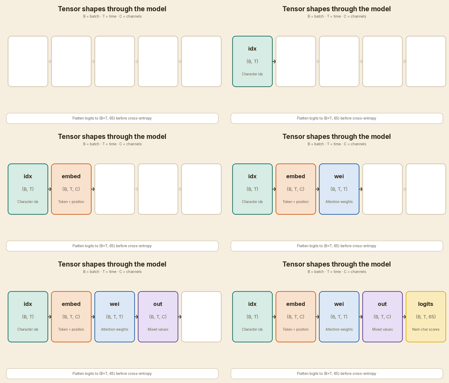
PyTorch comments in this repo use B, T, C.

Letter	Name	Meaning here
B	batch	How many independent windows sit in one GPU step
T	time / block	How many characters in one window (block_size)
C	channels	Width of a vector. For the bigram, C is 65 (vocab). For GPT, C is n_embd (384 in gpt.py)

Tensor	Shape	What is inside
idx / x	(B, T)	Character ids
y	(B, T)	Next-character ids (x, shifted by one)
token + position embed	(B, T, C)	One vector per character
attention weights	(B, T, T)	For each query position, a score on every key position
logits	(B, T, vocab_size)	Next-character scores
loss	scalar	Cross-entropy after flattening to (B*T, vocab_size)

---

1. Load tiny Shakespeare

The notebook starts by downloading the file, then reading it:

# Colab cell: download, then inspect
!wget https://raw.githubusercontent.com/karpathy/char-rnn/master/data/tinyshakespeare/input.txt

with open('input.txt', 'r', encoding='utf-8') as f:
    text = f.read()
print("length of dataset in characters: ", len(text))
print(text[:1000])

On that public file, len(text) is 1,115,394. About 1 MB. The first line is First Citizen:.

bigram.py and gpt.py skip the wget. They just open input.txt in the current folder. Download it once, then run the script.

---

2. chars, vocab_size, stoi / itos, encode / decode

chars = sorted(list(set(text)))
vocab_size = len(chars)
# 65 unique characters

stoi = {ch: i for i, ch in enumerate(chars)}
itos = {i: ch for i, ch in enumerate(chars)}
encode = lambda s: [stoi[c] for c in s]
decode = lambda l: ''.join([itos[i] for i in l])

print(encode("hii there"))
# [46, 47, 47, 1, 58, 46, 43, 56, 43]
print(decode(encode("hii there")))
# hii there

What this is doing:

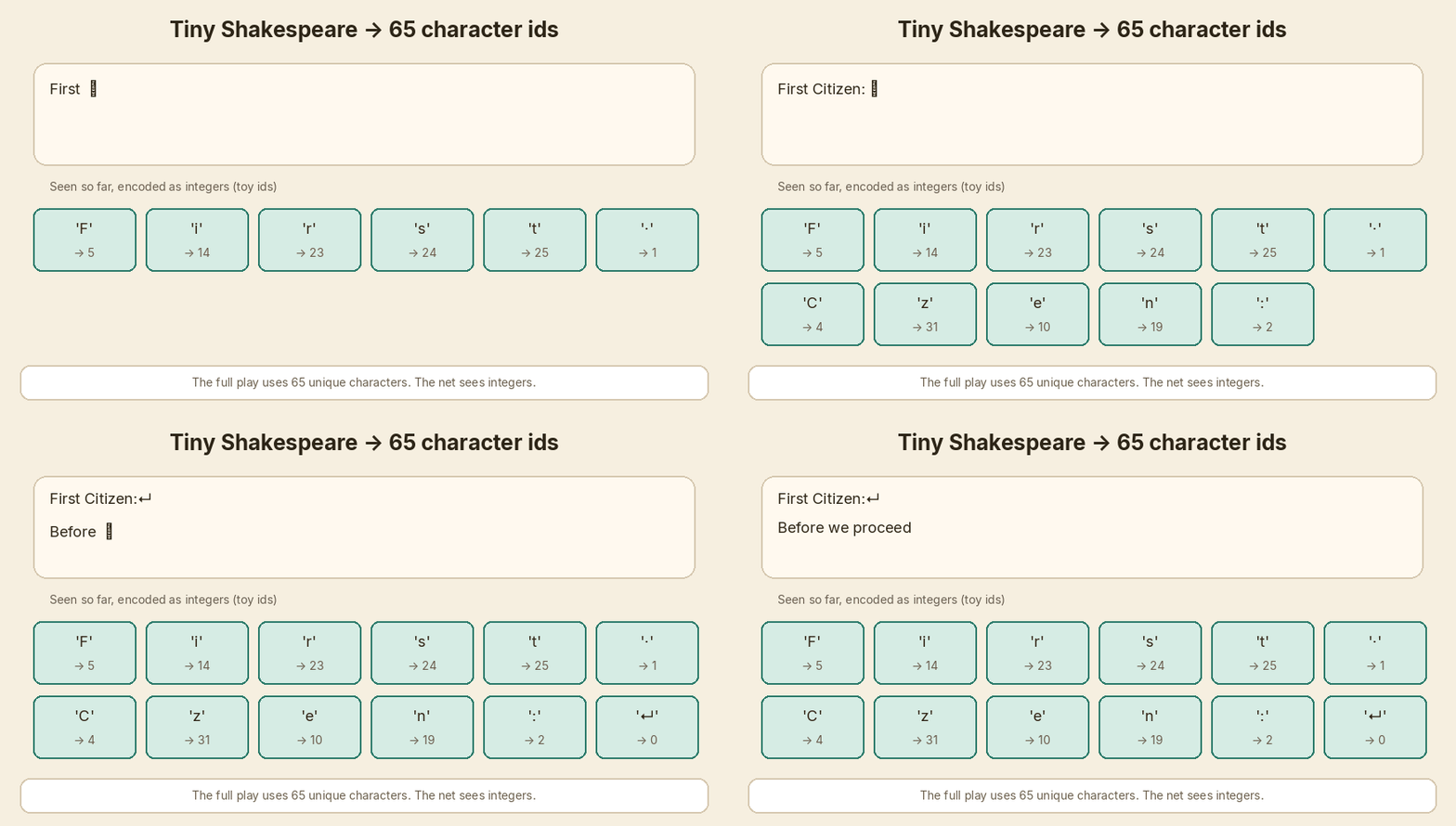
• set(text) = every unique character.
• sorted(...) = a stable alphabet. Newline comes first, then space, then punctuation, then letters.
• vocab_size is 65 on this file.
• stoi = string to integer. itos = integer to string.
• encode walks each character. decode joins them back.

The network never sees the letter h. It sees 46.

The parent post already explained why real ChatGPT-class models use subword tokenizers (tiktoken, SentencePiece) instead. Here we stay at one character = one token so the tensors stay readable.

---

3. One long tensor, then a 90/10 split

data = torch.tensor(encode(text), dtype=torch.long)
n = int(0.9 * len(data))  # first 90% train, rest val
train_data = data[:n]
val_data = data[n:]

• data is a 1-D torch.long tensor of length 1,115,394.
• First 90% is train. Last 10% is val.
• Val is for checking. Do not treat it as extra training text.

get_batch('train') and get_batch('val') pick from the matching slice.

---

4. block_size, batch_size, and get_batch

The notebook first sets block_size = 8 and prints one window:

x = train_data[:block_size]
y = train_data[1:block_size+1]
for t in range(block_size):
    context = x[:t+1]
    target = y[t]
    print(f"when input is {context} the target: {target}")

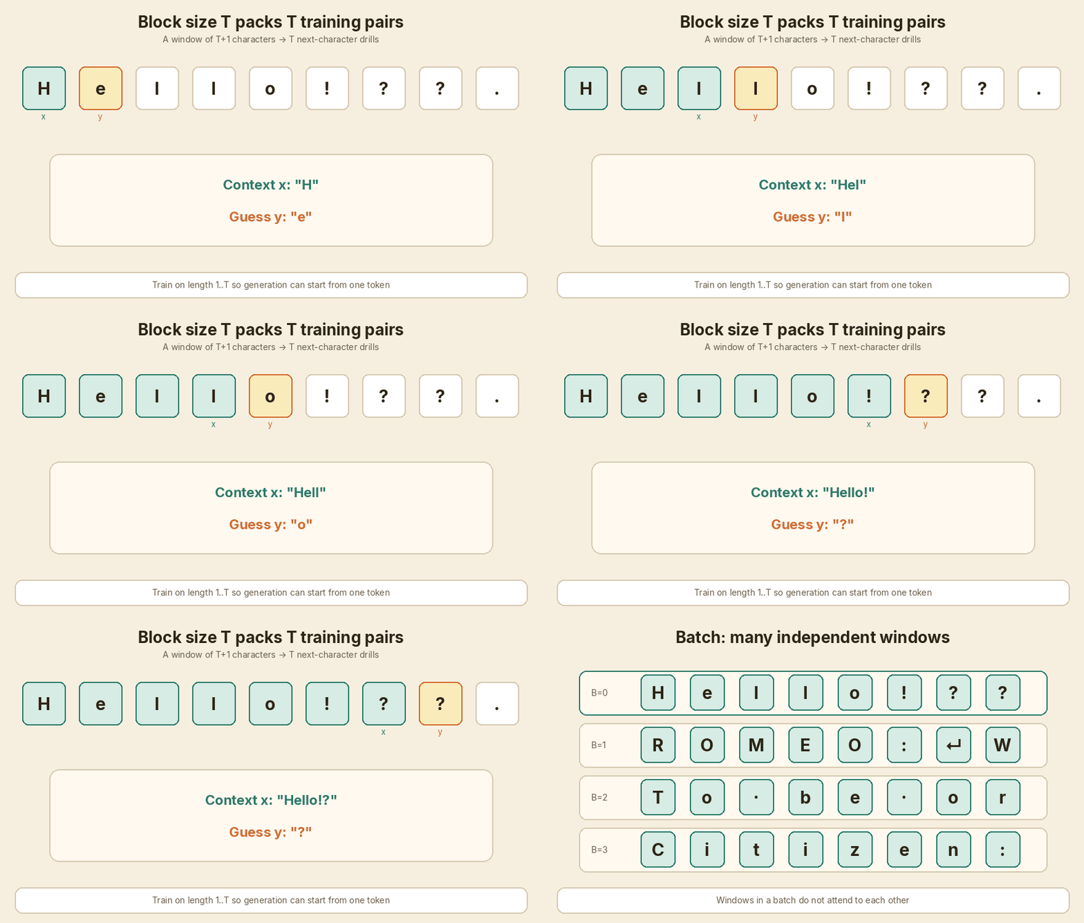
y is x shifted left by one. Every prefix of the window is a training example.

Worked example with letters (same rule as the notebook, easier to read than raw ids):

Step t	Context the model sees (x[:t+1])	Target (y[t])
0	H	e
1	He	l
2	Hel	l
3	Hell	o
4	Hello	!
5	Hello!	?
6	Hello!?	?
7	Hello!??	next char after the 8

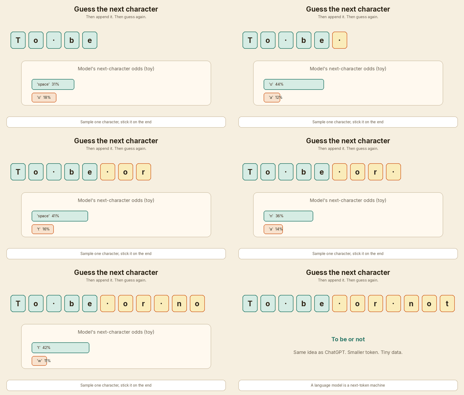
That is why a chunk of length T + 1 packs T predictions. Generation often starts from one token (the scripts start from a single 0, which decodes as newline). The model has to work with a short context, not only a full block.

Then the notebook builds a real batch:

batch_size = 4   # notebook walkthrough
block_size = 8

def get_batch(split):
    data = train_data if split == 'train' else val_data
    ix = torch.randint(len(data) - block_size, (batch_size,))
    x = torch.stack([data[i:i+block_size] for i in ix])
    y = torch.stack([data[i+1:i+block_size+1] for i in ix])
    return x, y

• Pick B random start indexes. Each start is far enough from the end that i + block_size still fits.
• x is characters [i : i+T].
• y is characters [i+1 : i+T+1].
• Stack them. Shapes are (B, T) and (B, T).

The scripts also move the batch to device (cuda if present, else cpu).

Windows in a batch do not attend to each other. That is the B dimension.

---

5. BigramLanguageModel: a lookup table

class BigramLanguageModel(nn.Module):
    def __init__(self, vocab_size):
        super().__init__()
        self.token_embedding_table = nn.Embedding(vocab_size, vocab_size)

    def forward(self, idx, targets=None):
        logits = self.token_embedding_table(idx)  # (B, T, C)
        if targets is None:
            return logits, None
        B, T, C = logits.shape
        logits = logits.view(B * T, C)
        targets = targets.view(B * T)
        loss = F.cross_entropy(logits, targets)
        return logits, loss

Plain reading:

• nn.Embedding(65, 65) is a 65×65 table.
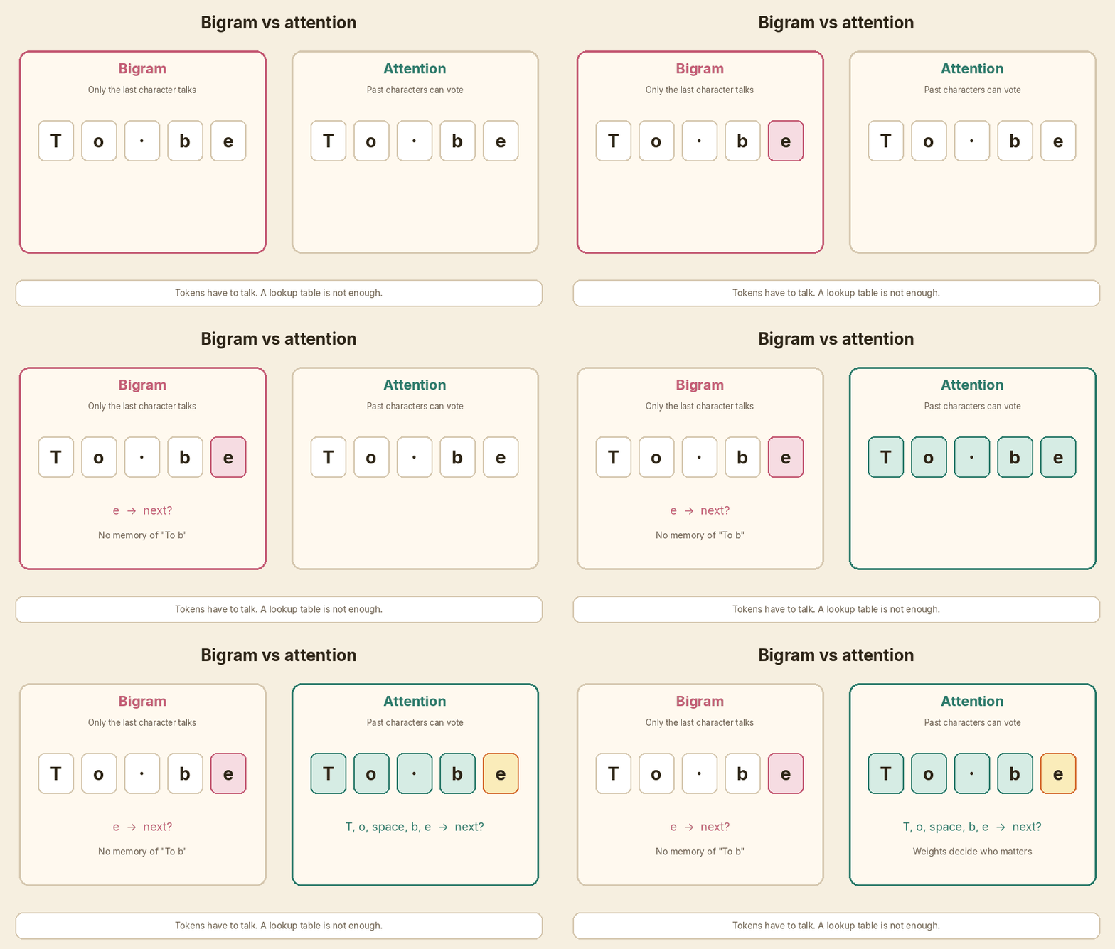
• Row 46 is the next-character scores after seeing id 46 (h).
• Tokens do not talk. Position 3 does not look at position 2.
• logits come out as (B, T, 65).
• F.cross_entropy wants (N, C) and a 1-D target of length N. So we flatten to (B*T, 65) and (B*T,).

Why the first loss is about 4.17

A fresh table is random. It has no reason to prefer e over q.

If every character is equally likely:

[ -\ln(1/65) \approx 4.17 ]

That is the “I have no idea” loss. The lecture’s trained bigram then sits around ~2.5. Those figures are from the lecture run, not from a stopwatch on my machine.

generate: softmax, then a dice roll

def generate(self, idx, max_new_tokens):
    for _ in range(max_new_tokens):
        logits, loss = self(idx)
        logits = logits[:, -1, :]          # (B, C) — last time step only
        probs = F.softmax(logits, dim=-1)  # (B, C)
        idx_next = torch.multinomial(probs, num_samples=1)
        idx = torch.cat((idx, idx_next), dim=1)
    return idx

• Take the last position’s 65 scores.
• Softmax turns them into probabilities that add to 1.
• torch.multinomial samples one id. Same prompt can give a different next character. That is on purpose.
• Append and repeat.

The bigram generate does not crop the context. It does not need to. There is no position table. gpt.py will crop. See below.

The scripts start generation from torch.zeros((1, 1)). Id 0 is newline in this alphabet.

---

6. The training loop

optimizer = torch.optim.AdamW(model.parameters(), lr=learning_rate)

for iter in range(max_iters):
    if iter % eval_interval == 0:
        losses = estimate_loss()
        print(f"step {iter}: train loss ... val loss ...")

    xb, yb = get_batch('train')
    logits, loss = model(xb, yb)
    optimizer.zero_grad(set_to_none=True)
    loss.backward()
    optimizer.step()

Line	What it does
AdamW(...)	The optimiser. It keeps a moving average of gradients and updates the table (and later, all the Linear layers)
zero_grad	Clear old gradients. set_to_none=True is a small PyTorch speed habit
backward	Compute gradients of loss w.r.t. every weight
step	Nudge the weights a little so the correct next character scores higher

estimate_loss is the honest meter:

@torch.no_grad()
def estimate_loss():
    out = {}
    model.eval()
    for split in ['train', 'val']:
        losses = torch.zeros(eval_iters)
        for k in range(eval_iters):
            X, Y = get_batch(split)
            logits, loss = model(X, Y)
            losses[k] = loss.item()
        out[split] = losses.mean()
    model.train()
    return out

• @torch.no_grad() = do not store gradients. Faster, less memory.
• model.eval() = turn dropout off (and any other train-only behaviour).
• Average eval_iters (200) random batches so one lucky batch does not fool you.
• model.train() = put dropout back before the next real update.

In the notebook’s first play cell, they train the bigram for 100 steps at lr=1e-3 just to see it move. bigram.py uses max_iters = 3000, lr = 1e-2, batch_size = 32.

---

7. The mathematical trick: three ways to average the past

The notebook section is titled The mathematical trick in self-attention. Goal:

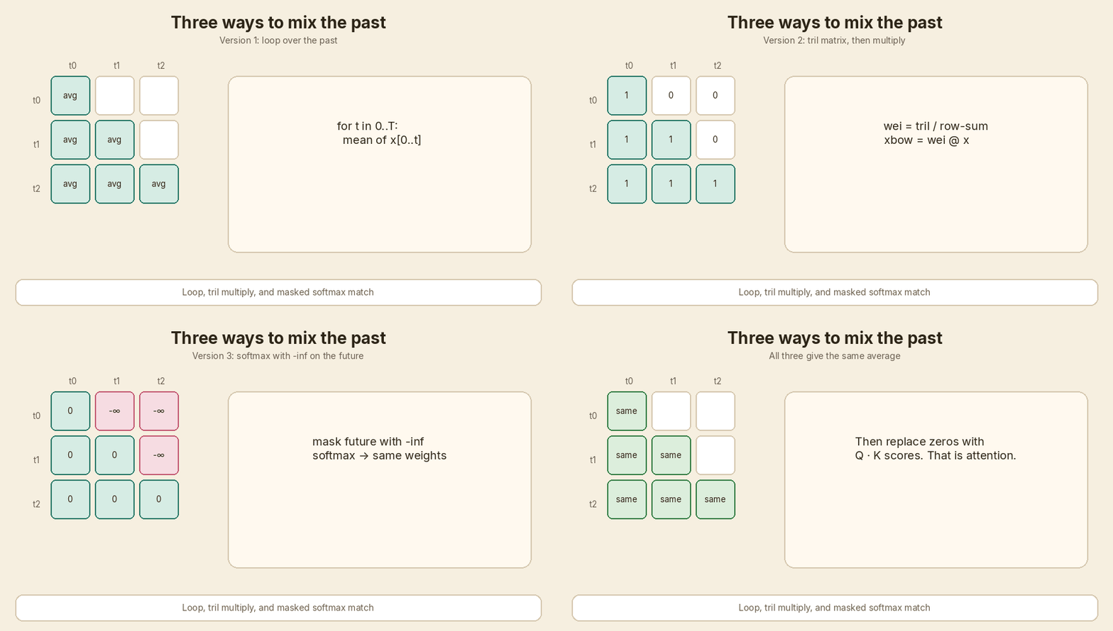
For each position t, mix information from positions 0..t. Do not look at the future.

Version 1 — a Python loop

# We want x[b,t] = mean_{i<=t} x[b,i]
xbow = torch.zeros((B, T, C))
for b in range(B):
    for t in range(T):
        xprev = x[b, :t+1]       # (t, C)
        xbow[b, t] = torch.mean(xprev, 0)

Correct. Slow. Fine for teaching.

Version 2 — torch.tril and one multiply

wei = torch.tril(torch.ones(T, T))
wei = wei / wei.sum(1, keepdim=True)
xbow2 = wei @ x   # (T, T) @ (B, T, C) -> (B, T, C)
# torch.allclose(xbow, xbow2) is True

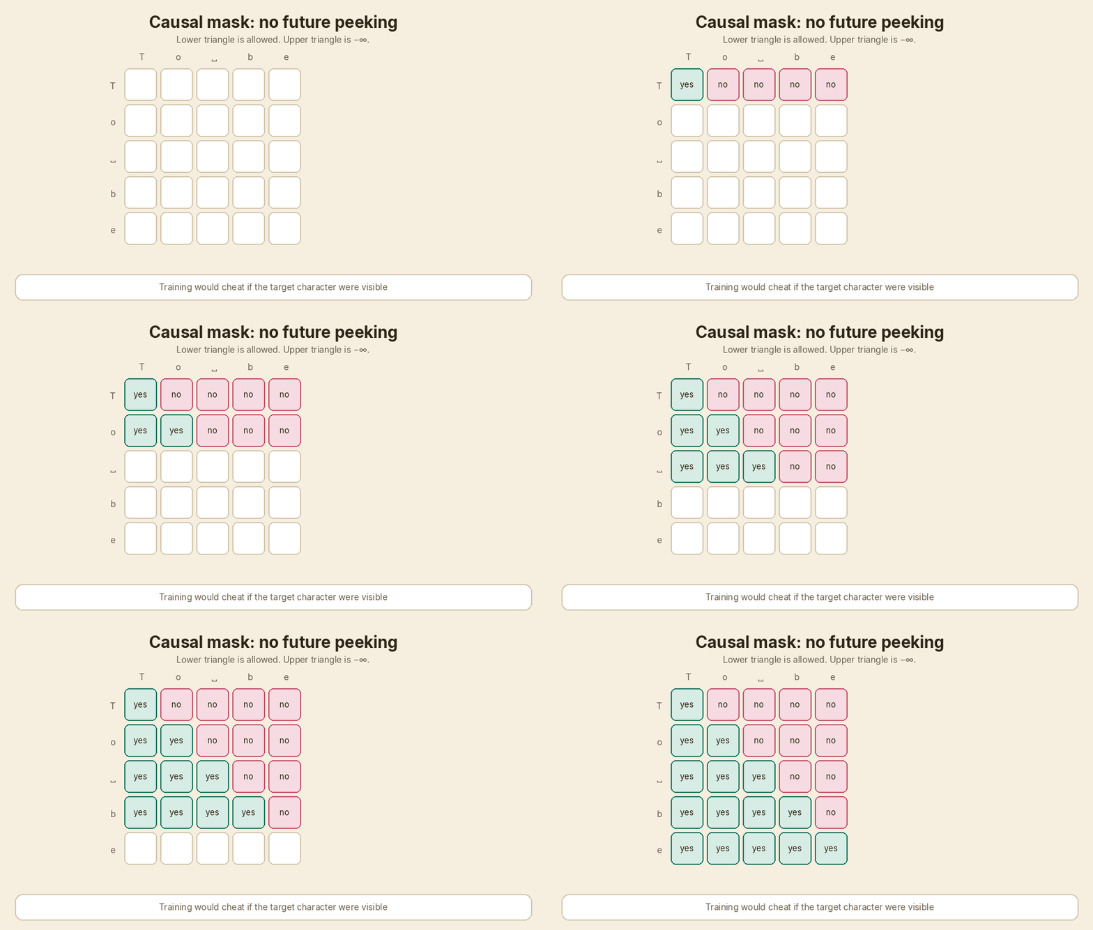
torch.tril is the lower triangle. 1s on and below the diagonal, 0s above. Divide each row by its sum and you get “average the past”. The @ does it for the whole batch at once.

Version 3 — softmax plus -inf

tril = torch.tril(torch.ones(T, T))
wei = torch.zeros((T, T))
wei = wei.masked_fill(tril == 0, float('-inf'))
wei = F.softmax(wei, dim=-1)
xbow3 = wei @ x
# torch.allclose(xbow, xbow3) is True

Softmax of 0 on the allowed cells, and -inf on the future, is the same uniform average. Softmax(-inf) is 0, so the future is gone.

All three tensors match. Version 3 is the one attention will use, because next we stop using zeros for wei and fill it with Query·Key scores instead.

---

8. One self-attention head

Notebook “version 4”, then the Head class in gpt.py. Same idea.

# Colab version 4 (toy sizes: B=4, T=8, C=32, head_size=16)
key = nn.Linear(C, head_size, bias=False)
query = nn.Linear(C, head_size, bias=False)
value = nn.Linear(C, head_size, bias=False)
k = key(x)    # (B, T, 16)
q = query(x)  # (B, T, 16)
wei = q @ k.transpose(-2, -1)  # (B, T, T)

tril = torch.tril(torch.ones(T, T))
wei = wei.masked_fill(tril == 0, float('-inf'))
wei = F.softmax(wei, dim=-1)
v = value(x)
out = wei @ v

gpt.py writes the scaled form and keeps a tril buffer:

wei = q @ k.transpose(-2, -1) * k.shape[-1]**-0.5
wei = wei.masked_fill(self.tril[:T, :T] == 0, float('-inf'))
wei = F.softmax(wei, dim=-1)
out = wei @ v

Piece	Shape	Job
x	(B, T, C)	Token (+ position) vectors
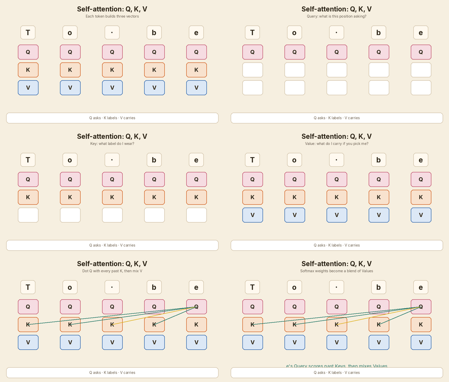
q, k, v	(B, T, head_size)	Ask / label / payload
wei before mask	(B, T, T)	Raw affinities
wei after softmax	(B, T, T)	Weights that sum to 1 along the last dim
out	(B, T, head_size)	Mixed values

Why divide by sqrt(head_size)

The notebook note is the clean version:

Scaled attention divides wei by 1/sqrt(head_size). When Q and K are unit variance, wei stays near unit variance. Softmax stays diffuse and does not saturate.

If you skip the scale, dots get large, softmax becomes almost one-hot, and the head only listens to one past token. The notebook shows this with softmax(scores) vs softmax(scores * 8).

[ \mathrm{Attention}(Q,K,V)=\mathrm{softmax}\left(\frac{QK^{\top}}{\sqrt{d}}+M\right)V ]

Encoder vs decoder, self vs cross

From the notebook notes, in the same words the lecture uses:

• Attention is a communication mechanism. Nodes in a graph mix information with a weighted sum.
• Attention has no notion of space. That is why we add position embeddings.
• Batch rows never talk to each other.
• Decoder block = keep the tril mask (language modelling).
• Encoder block = delete the mask line. Every token may look at every token. BERT-style.
• Self-attention = Q, K, V all come from x.
• Cross-attention = Q from x, K and V from another stream (the encoder, in the 2017 translation model).

The Colab even draws a French → English sketch: encode the source, then decode the target with a <START> token.

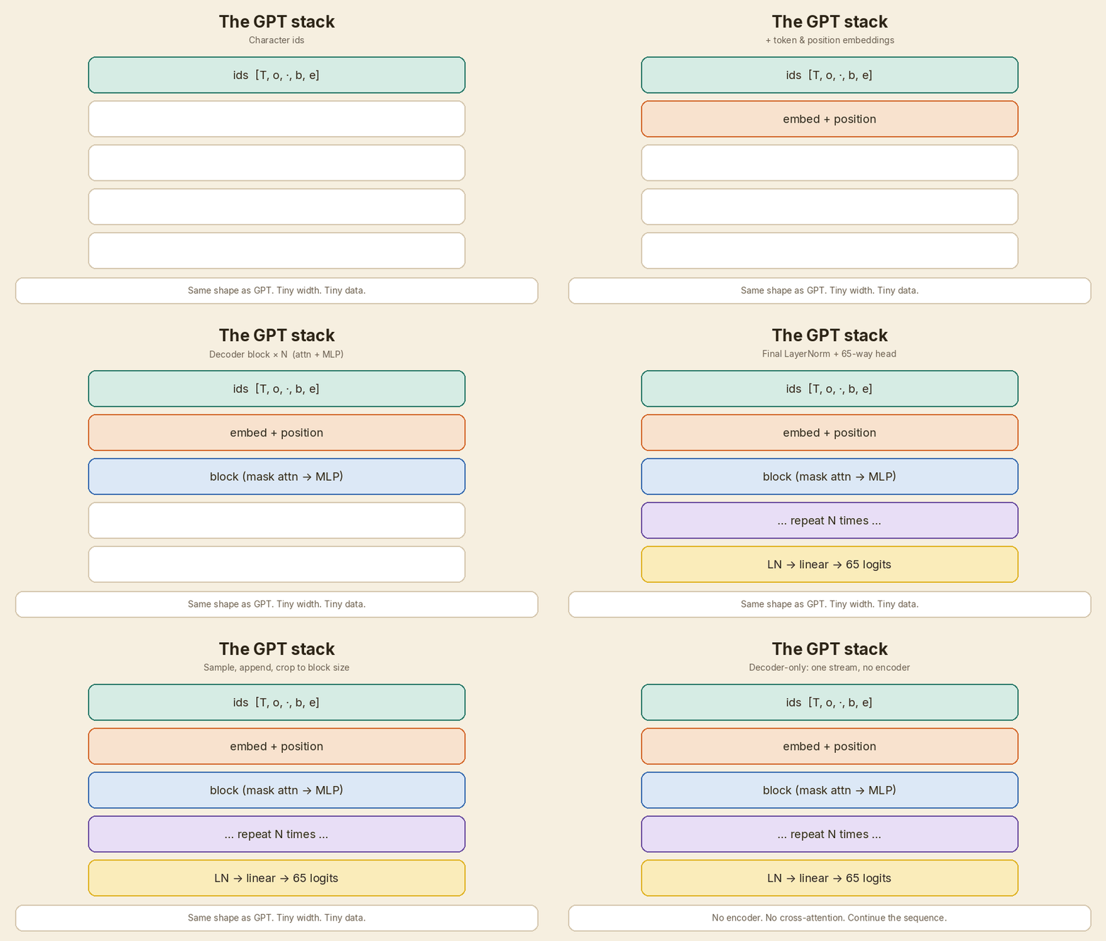
GPT in this repo is decoder-only. No encoder. No cross-attention.

---

9. Multi-head, feed-forward, and one Block

class MultiHeadAttention(nn.Module):
    def __init__(self, num_heads, head_size):
        super().__init__()
        self.heads = nn.ModuleList([Head(head_size) for _ in range(num_heads)])
        self.proj = nn.Linear(head_size * num_heads, n_embd)
        self.dropout = nn.Dropout(dropout)

    def forward(self, x):
        out = torch.cat([h(x) for h in self.heads], dim=-1)
        out = self.dropout(self.proj(out))
        return out

Several small heads run in parallel. Concat on the channel dim. Project back to n_embd. In gpt.py, n_embd = 384 and n_head = 6, so each head is size 64.

The class name in the repo is FeedFoward (one ‘r’). Search for that spelling.

class FeedFoward(nn.Module):
    def __init__(self, n_embd):
        super().__init__()
        self.net = nn.Sequential(
            nn.Linear(n_embd, 4 * n_embd),
            nn.ReLU(),
            nn.Linear(4 * n_embd, n_embd),
            nn.Dropout(dropout),
        )

Widen 4×, ReLU, project back. This runs per token. No mixing across time. Attention mixed. This thinks.

class Block(nn.Module):
    def forward(self, x):
        x = x + self.sa(self.ln1(x))
        x = x + self.ffwd(self.ln2(x))
        return x

That is the whole block:

1. LayerNorm.
2. Multi-head attention.
3. Add the residual (x + ...).
4. LayerNorm.
5. Feed-forward.
6. Add the residual again.

This is pre-norm: norm, then the sub-layer, then add. The 2017 paper drew post-norm. Pre-norm is what gpt.py uses.

flowchart TB
  x[x] --> ln1[ln1 LayerNorm]
  ln1 --> sa[Multi-head self-attention]
  sa --> add1["x = x + sa(...)"]
  add1 --> ln2[ln2 LayerNorm]
  ln2 --> ff[FeedFoward 4x + ReLU]
  ff --> add2["x = x + ff(...)"]

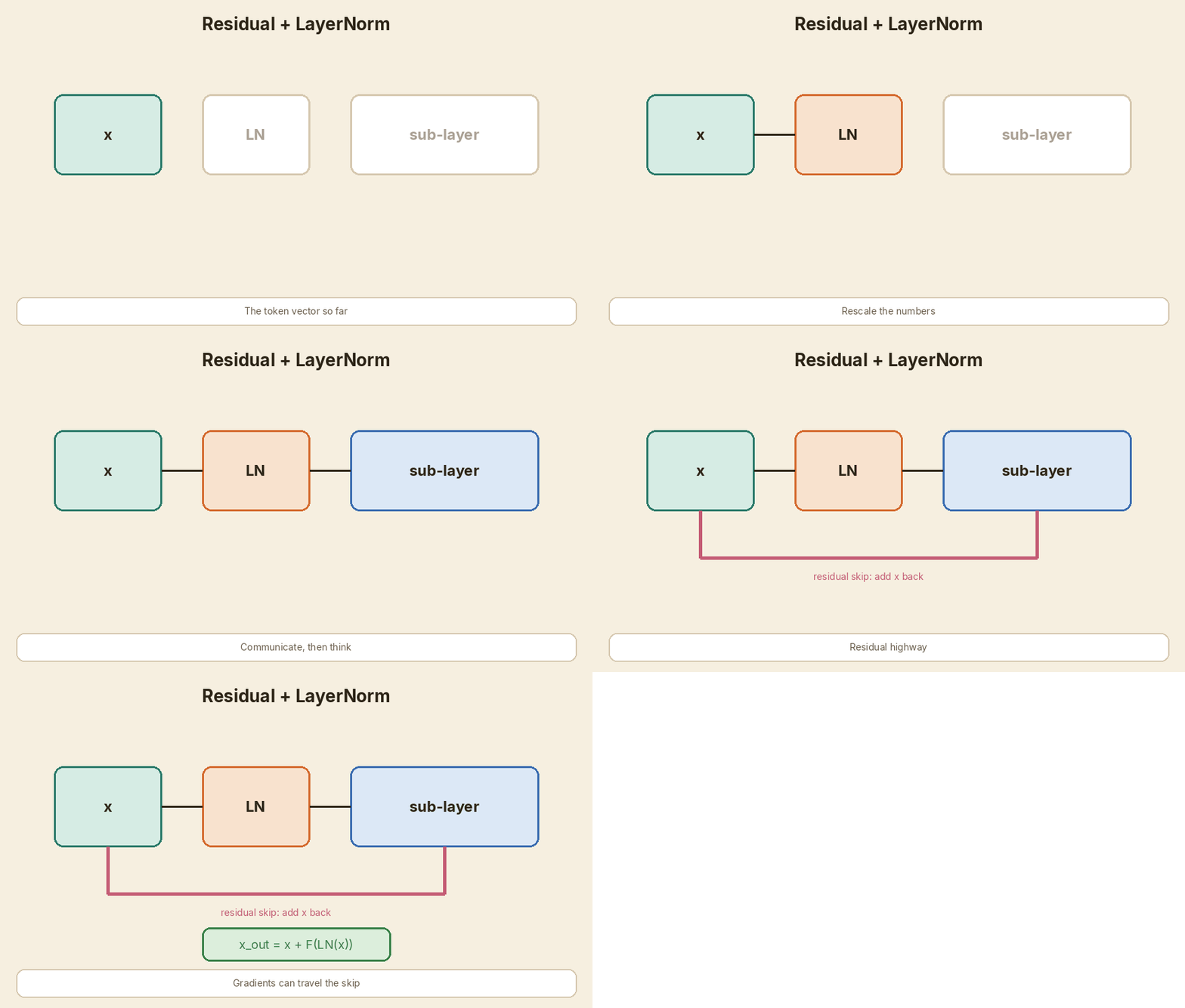
Dropout sits on attention weights, on the projection, and in the MLP. gpt.py uses dropout = 0.2.

---

10. Position embeddings, and why generate crops

Attention does not know order. If you swap two characters, the dots still run. So gpt.py adds a second table:

self.token_embedding_table = nn.Embedding(vocab_size, n_embd)
self.position_embedding_table = nn.Embedding(block_size, n_embd)

In forward:

tok_emb = self.token_embedding_table(idx)                         # (B, T, C)
pos_emb = self.position_embedding_table(torch.arange(T, device=device))  # (T, C)
x = tok_emb + pos_emb

“I am the letter e” plus “I sit at index 4”.

The position table only has block_size rows (256 in gpt.py). If the generated string grows past that, you cannot look up position 257. So generate crops:

idx_cond = idx[:, -block_size:]
logits, loss = self(idx_cond)

Keep the full story in idx (so you can decode the whole sample). Feed only the last 256 ids into the net.

The bigram script has no position table, so it does not crop.

---

11. gpt.py knobs

These are the values at the top of gpt.py. The lecture’s scaled run used this script.

Knob	gpt.py value	What it does
batch_size	64	Independent windows per step. Bigger = smoother gradients, more VRAM
block_size	256	Maximum characters the model may look at
max_iters	5000	How many AdamW steps
eval_interval	500	How often to print train/val loss
eval_iters	200	Batches averaged inside estimate_loss
learning_rate	3e-4	AdamW step size. Smaller than the bigram’s 1e-2
n_embd	384	Channel width C. Token and position vectors are this long
n_head	6	Parallel attention heads. Head size = 384 / 6 = 64
n_layer	6	How many Blocks are stacked
dropout	0.2	Fraction dropped in attention / projection / MLP
device	cuda if available else cpu	Where tensors live

The script prints sum(p.numel() for p in m.parameters())/1e6. That count is about 10.7M parameters.

The lecture reports a val loss around 1.48 after about 15 minutes on an A100. Those are the lecture’s numbers, not mine.

gpt.py also calls _init_weights (normal init, std 0.02). The repo README says this was not covered in the original video, and that nanoGPT’s model.py is the cleaner init story.

---

12. How to run it yourself

Colab

1. Open the lecture Colab.
2. File → Save a copy in Drive, so you are not writing to the shared notebook.
3. Runtime → Change runtime type → GPU (T4 is enough for the walkthrough cells).
4. Run from the top. The first cell wgets input.txt.
5. For the full finished cell at the bottom, expect minutes on a Colab GPU, not seconds. On CPU it will feel slow. Shrink n_layer, n_embd, and max_iters if the session is dragging.

Local scripts

wget https://raw.githubusercontent.com/karpathy/char-rnn/master/data/tinyshakespeare/input.txt
python bigram.py
python gpt.py

You need PyTorch. A GPU is optional for bigram.py. For gpt.py as written (6 layers, 384 width, 5000 steps), a laptop CPU will take a long time. I did not time it on this machine, so I will not invent a number.

Laptop CPU tips:

• n_layer = 2
• n_embd = 128 (keep it divisible by n_head)
• block_size = 64
• batch_size = 16
• max_iters = 500
• You will not hit the lecture’s 1.48 val loss. You will still see the loss drop and the samples get less random.

If you have a CUDA GPU, the scripts already pick device = 'cuda'.

---

13. Common gotchas

Symptom	Likely cause
RuntimeError about shape, often cross_entropy	Logits are still (B, T, C) and targets are (B, T). Flatten to (B*T, C) and (B*T,)
size of tensor a (257) must match size of tensor b (256) in generate	You forgot idx[:, -block_size:]. The position table only has block_size rows
Expected all tensors to be on the same device	Batch is on CPU, model is on CUDA (or the reverse). get_batch in the scripts calls .to(device). Do the same for context
Loss printed as nan	Learning rate too high, or -inf mask applied on the wrong dim. Check masked_fill uses tril[:T, :T]
Train loss keeps falling, val loss rises	Overfitting. 1 MB of Shakespeare and a 10M model can memorise. Dropout (0.2) is already there. You can also stop earlier
Samples look like Shakespeare but mean nothing	That is normal. The model copies local style (names, colons, thou). It is not thinking about the plot
FileNotFoundError: input.txt	The scripts do not download the file. wget it first, or run the Colab cell that does
Searching for FeedForward finds nothing	The class is spelled FeedFoward in this repo

---

14. bigram.py vs gpt.py

	bigram.py	gpt.py
Idea	Next-char lookup table	Decoder-only Transformer
batch_size	32	64
block_size	8	256
max_iters	3000	5000
learning_rate	1e-2	3e-4
Token embed	(65, 65) — already the logits	(65, 384)
Position embed	no	yes, 256 × 384
Attention	no	6 heads × 6 layers, causal mask
MLP	no	4× width, ReLU
Residual + LayerNorm	no	pre-norm in every block
Dropout	no	0.2
generate crop	no	idx[:, -block_size:]
Lecture-reported loss	~2.5 after a short train	~1.48 val on an A100 ~15 min
Parameters	tiny (65×65 plus nothing much)	about 10.7M

Same data. Same encode/decode. Same get_batch idea. The second file is “let the tokens talk”.

---

15. Where to go next

• Parent post (ideas only): How a tiny GPT learns
• Lecture video: Let’s build GPT: from scratch, in code, spelled out
• Cleaner, faster follow-on: karpathy/nanoGPT
• The 2017 paper: Attention Is All You Need
• Subword tokenizers, when you leave character-level: tiktoken

If you only change one thing after this walkthrough, print xb, yb, and wei[0] once. The rest of GPT is those three tensors, stacked.

---

Sources

• Colab — Building a GPT
• karpathy/ng-video-lecture (bigram.py, gpt.py, README; MIT)
• Tiny Shakespeare: char-rnn input.txt (1,115,394 characters, 65 unique, checked on that file)
• Zero to Hero
• Vaswani et al., Attention Is All You Need

Loss, wall-clock, and “about 10.7M” figures are from the lecture / gpt.py printout. Treat them as teaching examples.