Postgres EXPLAIN: Ask for the Plan
Your query feels slow.
Maybe it is looking up one order. Maybe it is scanning a large table.
Do not guess.
Do not add an index on every column “just in case.”
Ask Postgres for its plan.
flowchart LR
  A[Query feels slow] --> B[Ask for the plan]
  B --> C[Read the tree]
  C --> D[Watch the times]
That is the whole idea. The rest of this post is EXPLAIN vs ANALYZE, how JOINs work, how to read a plan tree, scan types, and a few numbers that actually matter.
Show me your plan
You can say:
Show me your plan before you start.
That is EXPLAIN.
Postgres writes the steps. It does not run the query yet.
You can also say:
Run the query. Then write how long each step took.
That is EXPLAIN ANALYZE.
Now Postgres really runs the query. Then it writes the real times.
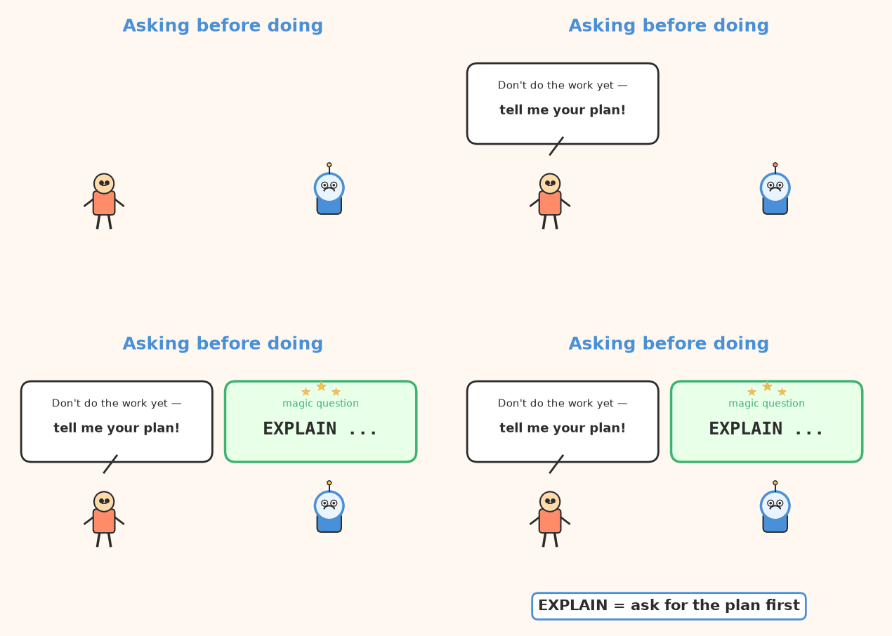
EXPLAIN is the plan. EXPLAIN ANALYZE is the plan plus the stopwatch.
There is a third ask.
Run the query. Write the times. And tell me which pages were already in memory, and which ones you fetched from disk.
That is EXPLAIN (ANALYZE, BUFFERS).
You get the plan, the stopwatch, and the page-fetch story.
Careful. ANALYZE does the work.
If the query only reads, it still has to walk the table. That can be slow. It can also take locks for a bit.
If the query changes things — DELETE, UPDATE — ANALYZE will really change the rows.
For this post, we only look. We do not change data.
EXPLAIN
SELECT *
FROM orders
WHERE user_id = 42;
EXPLAIN ANALYZE
SELECT *
FROM orders
WHERE user_id = 42;
EXPLAIN (ANALYZE, BUFFERS)
SELECT *
FROM orders
WHERE user_id = 42;
The first one is the plan.
The second one is walking the plan and writing the times.
The third one also counts pages already in memory versus pages fetched from disk.
How two tables meet
Sometimes the query needs two tables.
shops on the left. orders on the right. They match on shop_id.
A JOIN is how they combine.
When you JOIN, the plan tree grows a join node. Often Nested Loop, Hash Join, or Merge Join. That node combines the two child scans.
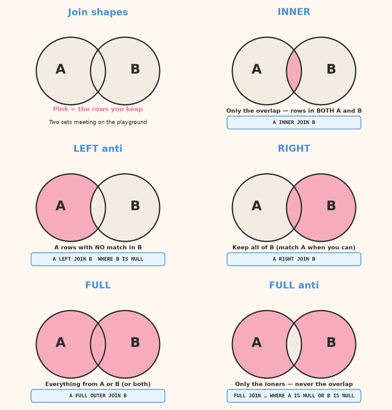
INNER       only the overlap
LEFT        all shops + matches
LEFT-ONLY   shops with no order
RIGHT       all orders + matches
RIGHT-ONLY  orders with no shop
FULL        everyone
FULL-ONLY   unmatched rows only
In the GIF, pink is the set of rows you keep.
Inner — only matching keys
SELECT s.name, o.id
FROM shops AS s
INNER JOIN orders AS o ON o.shop_id = s.id;
Keep a pair only when both tables share a key. Unmatched shops and unmatched orders stay out.
Left — every shop
SELECT s.name, o.id
FROM shops AS s
LEFT JOIN orders AS o ON o.shop_id = s.id;
Keep every shop. A matching order joins on. No order? The shop still sits there with NULLs on the order side.
Left-only — shops with no order
SELECT s.name
FROM shops AS s
LEFT JOIN orders AS o ON o.shop_id = s.id
WHERE o.id IS NULL;
Keep shops whose order side is NULL. The empty side is the point.
Right — every order
SELECT s.name, o.id
FROM shops AS s
RIGHT JOIN orders AS o ON o.shop_id = s.id;
Keep every order. A matching shop joins on. No shop? The order still sits there with NULLs on the shop side.
Right-only — orders with no shop
SELECT o.id
FROM shops AS s
RIGHT JOIN orders AS o ON o.shop_id = s.id
WHERE s.id IS NULL;
Keep orders whose shop side is NULL. Orphan orders. No matching shop.
Full — everyone
SELECT s.name, o.id
FROM shops AS s
FULL OUTER JOIN orders AS o ON o.shop_id = s.id;
Keep every shop and every order. Matches join. Unmatched rows still sit with NULLs.
Full-only — unmatched rows
SELECT s.name, o.id
FROM shops AS s
FULL OUTER JOIN orders AS o ON o.shop_id = s.id
WHERE s.id IS NULL OR o.id IS NULL;
Drop the matched pairs. Keep only the unmatched shops and the unmatched orders.
The join shape is your question. The join node is how Postgres does the work. Look at that node in the tree next.
The plan is a tree
The plan is not one long sentence.
It is a tree.
Big step on top. Little steps tucked under it.
The little steps fetch the rows. The big step combines them.
Start from the inside. Start from the bottom.
That is where Postgres first touches the tables.
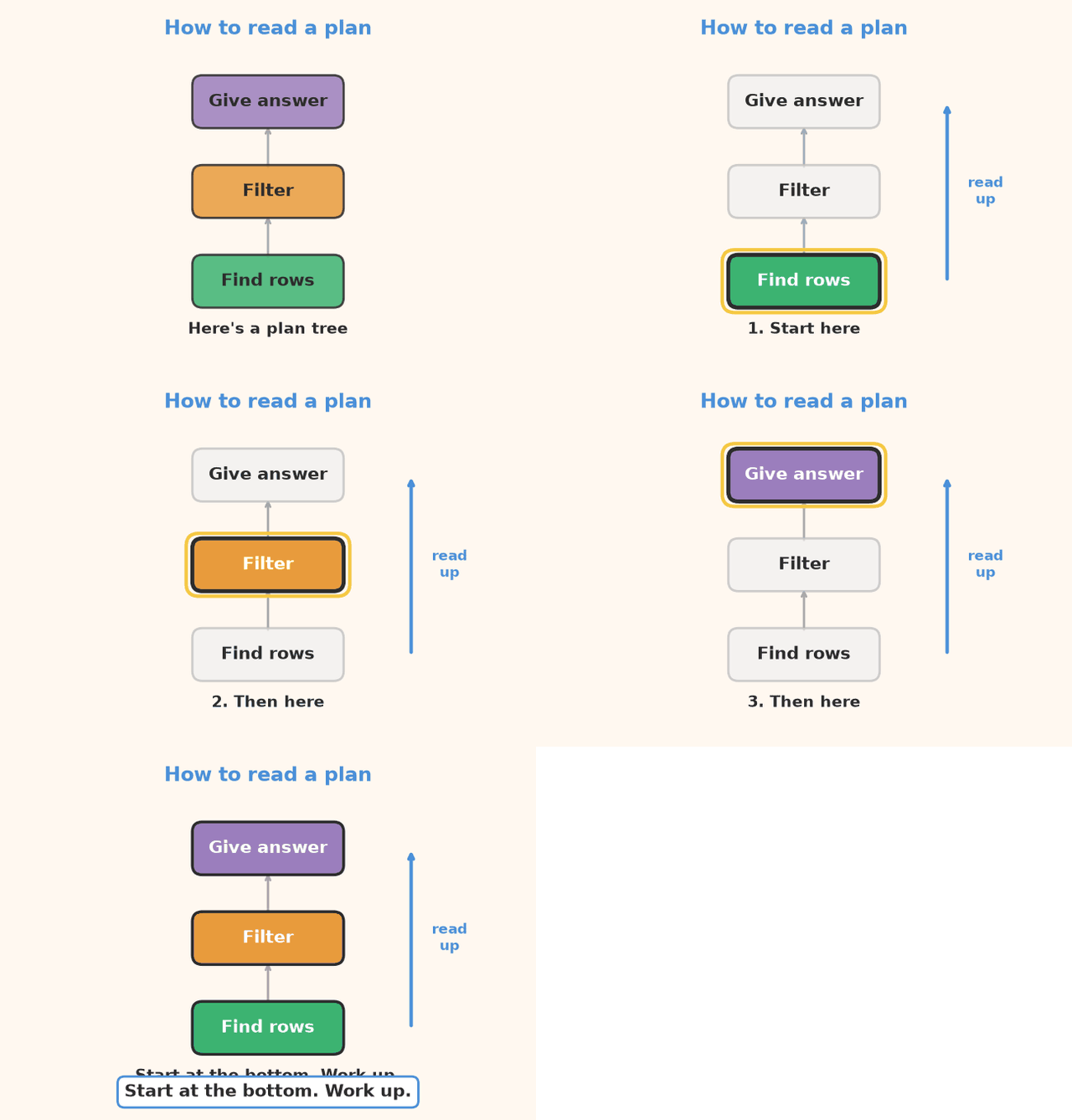
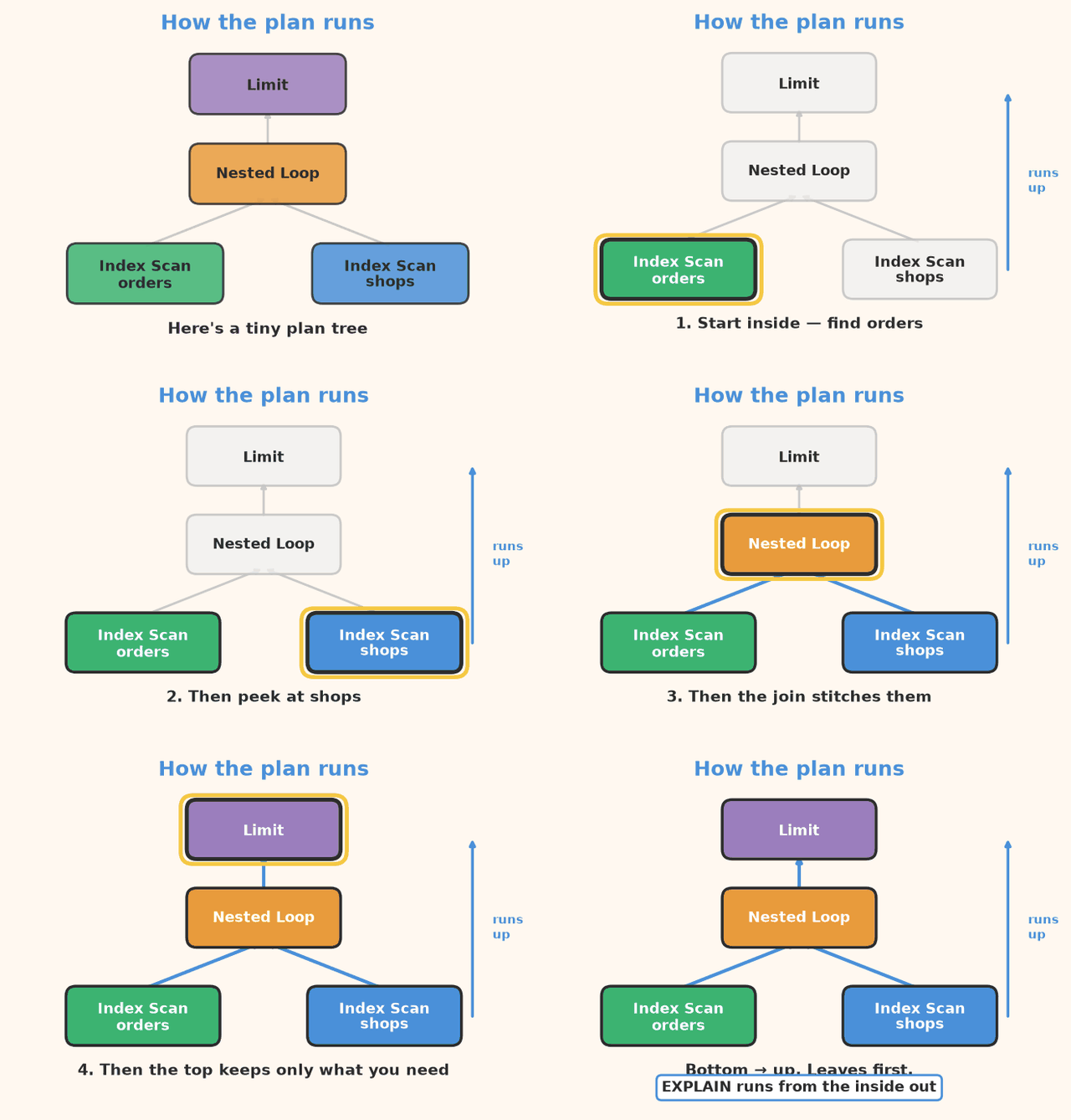
flowchart TB
  L[Look up orders] --> J[Join]
  U[Look up users] --> J
  J --> T[Return rows]
Read it like this:
- What did it do on
orders? - What did it do on
users? - How did it join those tables? That middle box is the join node.
- Then look at the top. A Limit can sit there: “stop when you have one yes.”
Each box is a node. A node is one job.
Look at the name of the job first. Then look at the numbers.
How it looks things up
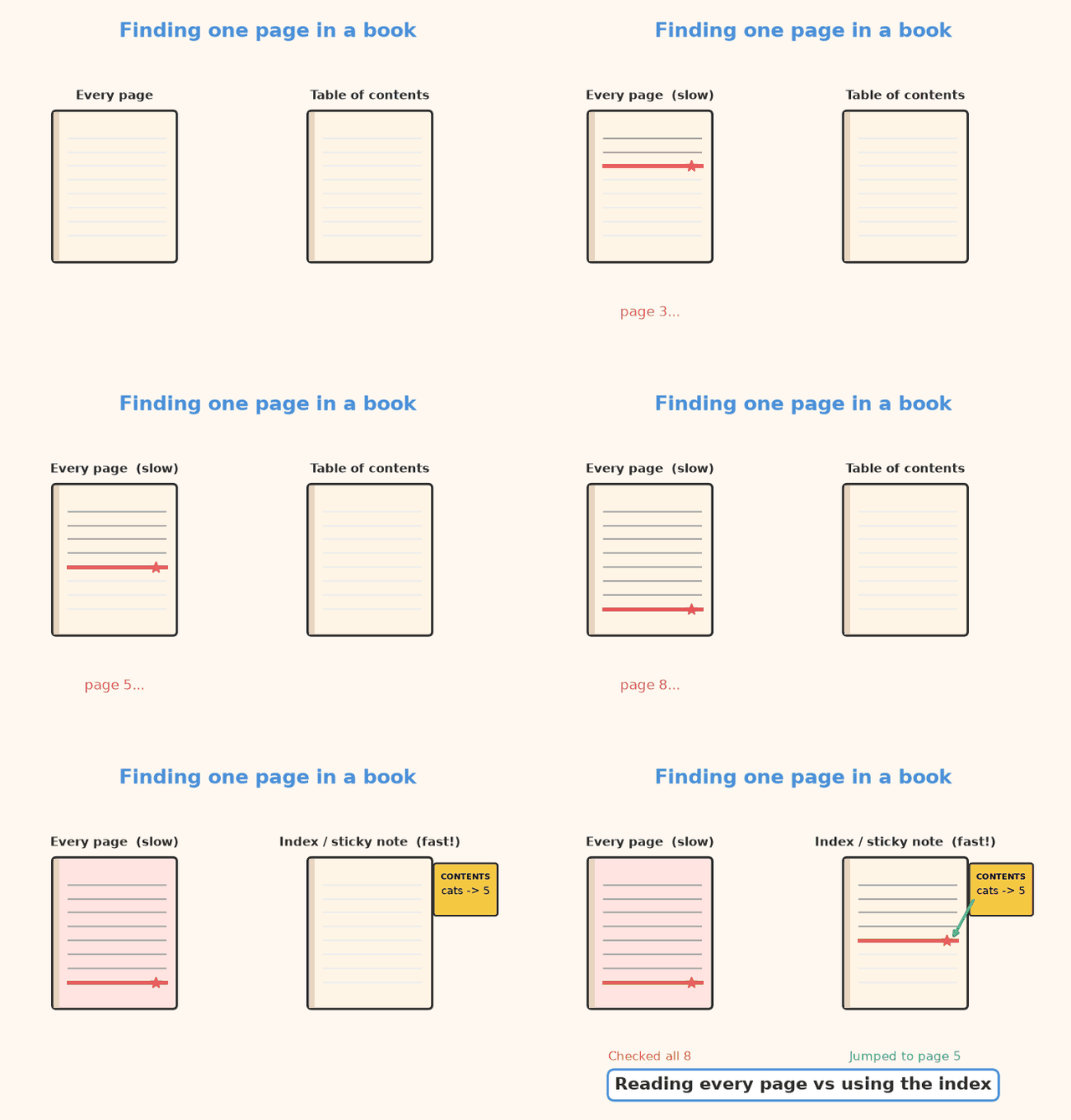
A table is stored in pages. Each page is a chunk of rows.
Read every page
Seq Scan means: walk the whole table.
Every page. Every row. Then keep the ones that match.
That is fine for a small table.
That is a long walk for a huge table when you only want one row.
Use an index
An index is a lookup structure.
“user_id 42 lives on these pages.”
Index Scan means: check the index. Then fetch those heap pages.
Index Only Scan is even shorter. The answer is already in the index. You do not visit the heap.
Collect page numbers, then one trip
Sometimes many rows match. The index lists lots of page numbers.
Bitmap Heap Scan means: collect the page numbers. Sort them. Then visit each page once.
You do not run back to the same page ten times.
Bitmap first. Then one pass over the heap.
| What you see | What Postgres did |
|---|---|
| Walk every page | Seq Scan |
| Index, then the heap | Index Scan |
| Answer already in the index | Index Only Scan |
| Collect page numbers, then fetch | Bitmap Heap Scan |
Numbers on the page
A plan line looks busy. You only need a few numbers.
Here is a tiny made-up line:
Index Scan using orders_user_id_idx on orders
  (cost=0.29..8.31 rows=3 width=84)
  (actual time=0.018..0.021 rows=3 loops=1)
  Index Cond: (user_id = 42)
Guessed rows vs real rows
rows=3 on the first line is the guess.
Postgres guessed: “about 3 orders.”
After ANALYZE, rows=3 on the actual line is the truth.
If the guess said 3 and the truth was 30,000, raise a flag.
The estimate was wrong. The plan may be the wrong plan.
Cost
Cost is “how hard it looks on paper.”
It is not seconds. It is Postgres comparing two plans.
The first number is startup cost. Work before the first answer row.
The second number is total cost. Work to finish the whole job.
A cheap-looking plan can still be the wrong one if the row guess is bad.
Actual time
Actual time is the stopwatch. It is milliseconds.
The first number is startup. Time to the first row.
The second number is total. Time to the last row.
If you only needed the first ten answers, startup matters a lot.
Loops
Loops means: “I did this step again and again.”
Same inner scan, once for every outer row.
The time on the line is per loop.
So 2 ms × 10,000 loops is a long day.
Guessed rows. Real rows. Paper cost. Real time. How many times.
Indexes that help
An index is useful when the plan actually uses it.
You can tell it was used when the node says Index Scan, Index Only Scan, or Bitmap Index Scan.
You can often see the name: orders_user_id_idx.
This is the missing-index flag:
- big table
- you wanted one row, or a few rows
- the plan says Seq Scan
- then a Filter throws almost everyone away
That is “read the whole table, then keep one row.”
Do not put an index on every column.
Every new write must update those indexes. Writes get slower. Unused indexes waste space.
Add an index when a real plan shows a long scan you can skip. Then ask for the plan again.
CREATE INDEX orders_user_id_idx ON orders (user_id);

EXPLAIN
SELECT id, created_at
FROM orders
WHERE user_id = 42;
Where the clock is
Do not only look at the last line.
Find the node with the big actual time.
That is the slow step.
Startup is time until the first row comes out.
Total is time until the whole job is done.
A sort can sit there a long time before the first row comes out. The pile has to be ordered first.
A scan can drip rows out early. Startup is small. Total still grows if the table is long.
Ask:
Which node ate the clock? Was it waiting to start, or working the whole time?
Raise a flag
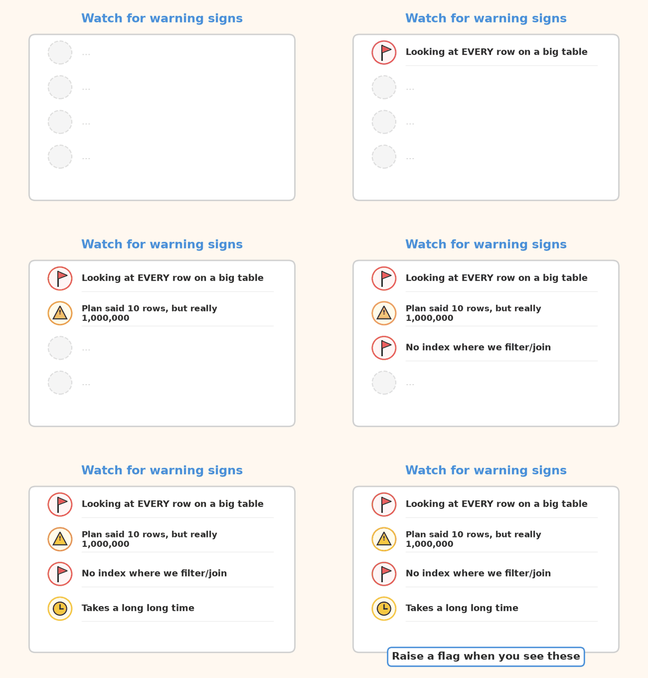
Check this list. One flag is a clue. Two flags is a loud clue.
- Seq Scan on a large table when you expected a lookup. “Find user 42” should not read every page.
- Huge gap between guessed rows and real rows. The estimate was wrong, so the plan may be wrong.
- Many loops on a node that is already slow. Same hard step, thousands of times.
- Sort or Hash ran out of work_mem. The working set did not fit in memory. Postgres spilled to disk. That extra shuffle is slow.
- Filter that throws away almost every row after a wide scan. It already walked the whole table. Then it said no to nearly everyone.
- Many Rows Removed by Filter after an Index Scan already found candidates. The index did its job. Then a later rule threw the rows away. The fetch already happened. Try to push that rule into Index Cond — a better index, or a simpler query.
A Seq Scan is not always bad. A tiny table? Read the whole thing. That can be the smart plan.
The flag is when the table is huge and you only wanted a few rows.
A tiny safe example
Pretend two tables. users. orders.
We only look. We do not change any rows.
EXPLAIN
SELECT u.name, o.id
FROM users AS u
JOIN orders AS o ON o.user_id = u.id
WHERE u.id = 42;
Same query, now with the stopwatch:
EXPLAIN ANALYZE
SELECT u.name, o.id
FROM users AS u
JOIN orders AS o ON o.user_id = u.id
WHERE u.id = 42;
Read the tree from the inside.
Did users use an index for id = 42?
Did orders use an index on user_id?
Or did one side read every page?
Then look at guessed rows vs real rows. Then look at the times.
A permission check that looks simple
The tiny example asked for names.
This one only asks: may this shopper see this one order?
Yes or no. One row. Or no row.
It looks like a small check. The plan can still be a tall tree.
Pretend a shop. Fake tables: orders, shops, shoppers, clubs, shop admins.
Fake IDs. We only look.
EXPLAIN (ANALYZE, BUFFERS)
SELECT 1
FROM orders AS o
JOIN shops AS s
  ON s.id = o.shop_id
JOIN shoppers AS c
  ON c.id = o.shopper_id
WHERE o.id = 1001
  AND s.region_id = 42
  AND (
    COALESCE((s.settings ->> 'open_late')::boolean, false)
    OR EXISTS (
      SELECT 1
      FROM club_members AS cm
      JOIN clubs AS cl
        ON cl.id = cm.club_id
      WHERE cm.shopper_id = o.shopper_id
        AND cl.shop_id = s.id
    )
    OR EXISTS (
      SELECT 1
      FROM shop_admins AS sa
      WHERE sa.shop_id = s.id
        AND sa.shopper_id = 7
    )
  )
LIMIT 1;
That query has three permission rules. Any one yes is enough.
- The shop settings say
open_late. - Or this shopper is in a club for that shop.
- Or shopper
7is an admin at that shop.
LIMIT 1 and SELECT 1 mean: “I only need a yes.”
Postgres wrote a tree like this. I shortened it. The names are toy names.
Limit  (cost=0.86..9.20 rows=1 width=4) (actual time=0.412..0.413 rows=0 loops=1)
  Buffers: shared hit=18 read=4
  I/O Timings: shared read=0.186
  ->  Nested Loop  (cost=0.86..9.20 rows=1 width=4) (actual time=0.411..0.411 rows=0 loops=1)
        ->  Nested Loop  (cost=0.58..8.90 rows=1 width=8) (actual time=0.410..0.410 rows=0 loops=1)
              ->  Index Scan using orders_pkey on orders o
                    (cost=0.29..8.31 rows=1 width=12)
                    (actual time=0.016..0.017 rows=1 loops=1)
                    Index Cond: (id = 1001)
                    Buffers: shared hit=3
              ->  Index Scan using shops_id_region_deleted_at on shops s
                    (cost=0.29..0.58 rows=1 width=8)
                    (actual time=0.390..0.390 rows=0 loops=1)
                    Index Cond: ((id = o.shop_id) AND (region_id = 42))
                    Filter: (COALESCE(((settings ->> 'open_late'::text))::boolean, false)
                             OR (hashed SubPlan 1)
                             OR (hashed SubPlan 3))
                    Rows Removed by Filter: 1
                    Buffers: shared hit=15 read=4
                    I/O Timings: shared read=0.186
                    SubPlan 1
                      ->  Hash Join  (cost=8.60..16.90 rows=1 width=0)
                            (actual time=0.210..0.212 rows=0 loops=1)
                            Hash Cond: (cm.club_id = cl.id)
                            ->  Index Scan using club_members_shopper_id_idx
                                  on club_members cm
                                  Index Cond: (shopper_id = o.shopper_id)
                            ->  Hash
                                  ->  Index Only Scan using clubs_pkey on clubs cl
                                        Index Cond: (id = cm.club_id)
                                        Heap Fetches: 0
                    SubPlan 3
                      ->  Index Only Scan using shop_admins_shop_id_shopper_id_key
                            on shop_admins sa
                            (actual time=0.018..0.018 rows=0 loops=1)
                            Index Cond: ((shop_id = s.id) AND (shopper_id = 7))
                            Heap Fetches: 0
        ->  Index Scan using shoppers_pkey on shoppers c
              (cost=0.28..0.30 rows=1 width=4)
              (never executed)
Planning Time: 1.842 ms
Execution Time: 0.468 ms
flowchart TB
  O[Find the order] --> S[Find the shop]
  S --> F{Permission rules}
  F -->|fail| X[Zero rows. Stop.]
  F -->|pass| C[Then look up the shopper]
Read it from the inside.
Index Cond vs the later Filter
Index Cond is the lookup in the index.
On orders, it jumped to id 1001. That is the primary key. One row.
On shops, it jumped with two clues: shop id and region 42.
Look at the index name: shops_id_region_deleted_at.
That is one index with more than one column. A composite index. It helped the join and the region rule.
Filter is the later rule. It runs after the index already found a candidate.
Here the Filter is the permission check: open_late or club or admin.
Rows Removed by Filter: 1 means: the index did find a shop. Then the permission check said no.
The fetch of that shop already happened. Then the row was dropped.
If you see lots of rows removed this way, the expensive work happened before the Filter. Try to push that rule into Index Cond — a better index, or a simpler query.
Side queries under the Filter
Those EXISTS checks show up as SubPlan 1 and SubPlan 3.
A SubPlan is a nested query. “Check the club table. Check the admin table.”
Because the rules are joined with OR, Postgres may run those SubPlans for each shop row that reaches the Filter.
SubPlan 1 is a Hash Join. It takes an Index Scan on club_members and an Index Only Scan on clubs. Two small inputs. Then it matches club ids.
SubPlan 3 is shorter. One Index Only Scan on shop_admins. The admin lookup used a two-column index: shop id plus shopper 7.
Index Only Scan means the answer was already in the index.
Heap Fetches: 0 means: it did not visit the heap. Zero heap trips. That is the cheap kind.
For each outer row, probe the inner side
See the two Nested Loop boxes stacked up?
That is the join node from the two-tables section. A Nested Loop means: for each row from the outer step, probe the inner step.
- Outer: find order
1001. One row. - Inner: use that order’s shop id. Probe
shops. - That Nested Loop feeds another Nested Loop. The next probe would be
shoppers.
One order. Then that order’s shop. Then that shop’s shopper.
It is not “dump both tables and mix.” It is probe, probe, probe.
A join it never ran
The last line says Index Scan on shoppers… (never executed).
Do not panic.
The shop step already returned zero rows. The permission check failed. So Postgres skipped the shopper lookup.
That is a short-circuit. An earlier step already finished the story, so the later join never ran.
A node that never ran is often a clue that an earlier step already decided.
Pages in memory vs disk
Buffers: shared hit=18 read=4 is the page-fetch story.
- shared hit = that page was already in memory (shared buffers).
- shared read = Postgres had to fetch it from disk.
I/O Timings: shared read=0.186 is how long the disk reads took.
Hits are cheap. Reads can be slow. A tiny query can still wait on disk.
Zero rows, but you still learned
The plan guessed rows=1. “Maybe a yes.”
The truth was actual rows=0. The permission check failed.
You can still see where the row died: Rows Removed by Filter: 1 on shops.
The top box is a Limit. “Stop when you have one yes.” Cheap when the indexes hit. You still watch the Filter and the SubPlans.
Now look at the last two lines.
Planning Time: 1.842 ms.
Execution Time: 0.468 ms.
Planning the query took longer than running it.
That can happen on a tiny query. The walk was short. Building the plan was the slow part. Do not only stare at Execution Time.
The index found the shop. A later Filter said no. Then Postgres stopped probing other tables.
Terms used in this post
You do not need this table to follow the examples. It is only a quick lookup.
| Term | Meaning |
|---|---|
| EXPLAIN | The plan, no work yet |
| EXPLAIN ANALYZE | Run the query and time it |
| EXPLAIN (ANALYZE, BUFFERS) | Plan, stopwatch, and page-fetch story |
| plan node | One job in the tree |
| Seq Scan | Read every page |
| Index Scan | Index lookup, then the heap |
| Index Only Scan | Answer already in the index |
| Bitmap Index Scan + Bitmap Heap Scan | Collect page numbers, then fetch once |
| Index Cond | Lookup condition used by the index |
| Filter | Later rule, after a candidate is found |
| Rows Removed by Filter | Rows the later rule threw away |
| SubPlan | Nested query (often an EXISTS) |
| Buffers | shared hit = in memory; shared read = from disk |
| never executed | This node was skipped |
| JOIN | Combine two tables (inner / left / right / full) |
| anti | WHERE the other key IS NULL |
| Nested Loop | For each outer row, probe the inner side |
| Hash Join | Build a hash table, then probe it |
| Merge Join | Walk two sorted inputs |
| cost | Paper difficulty (startup .. total) |
| rows | Estimated row count |
| actual time | Stopwatch (ms, per loop) |
| loops | How many times this node ran |
| external merge / hash batches | Disk spill when work_mem is too small |
In short
Don’t guess why it is slow. Ask for the plan. Read the tree from the inside. If two tables join, look at the join node. Check whether an index was used. Watch the times. If a Filter throws a row away, look at Index Cond versus the later rule.
If this helped:

Discussion
Reactions and replies via GitHub Discussions. Sign in with GitHub to comment.