From a Sentence to ChatGPT
ChatGPT answers in full sentences. The machine does not start there.
It starts with pieces of text, lists of numbers, a compare-and-mix step called attention, a stack of the same block, and a lot of “guess the next word” training.
This post is that ladder. One chain of If you do X, you get Y. Same sentence the whole way: The bus is late.
The IDs below are toy numbers I made up. They are not from GPT-2, tiktoken, or any real vocab. The matrices are tiny on purpose. You can type the NumPy as you read, or run code/build_along.py (seed 7) and get the same prints.
If you want the bigger-picture story — a small GPT trained on Shakespeare characters — read How a Tiny GPT Learns. This page is the same idea, one checkpoint at a time.
flowchart TB
  A[Sentence] --> B[Tokens + toy IDs]
  B --> C[Embeddings x]
  C --> D[Query / Key / Value]
  D --> E[Scores]
  E --> F[Softmax weights]
  F --> G[Context vector]
  G --> H[Self-attention]
  H --> I[One transformer block]
  I --> J[Stack of blocks]
  J --> K[Next-word chat model]
  K --> L[Back to the sentence]
Shared setup for every snippet:
import numpy as np

np.random.seed(7)
np.set_printoptions(precision=2, suppress=True)

def softmax(x, axis=-1):
    e = np.exp(x - np.max(x, axis=axis, keepdims=True))
    return e / e.sum(axis=axis, keepdims=True)

SENTENCE = "The bus is late"
TOKENS = ["The", "bus", "is", "late"]
IDS = np.array([11, 42, 7, 88])  # toy IDs, not a real vocab
D = 4
SCALE = np.sqrt(D)
1. Break a sentence into pieces
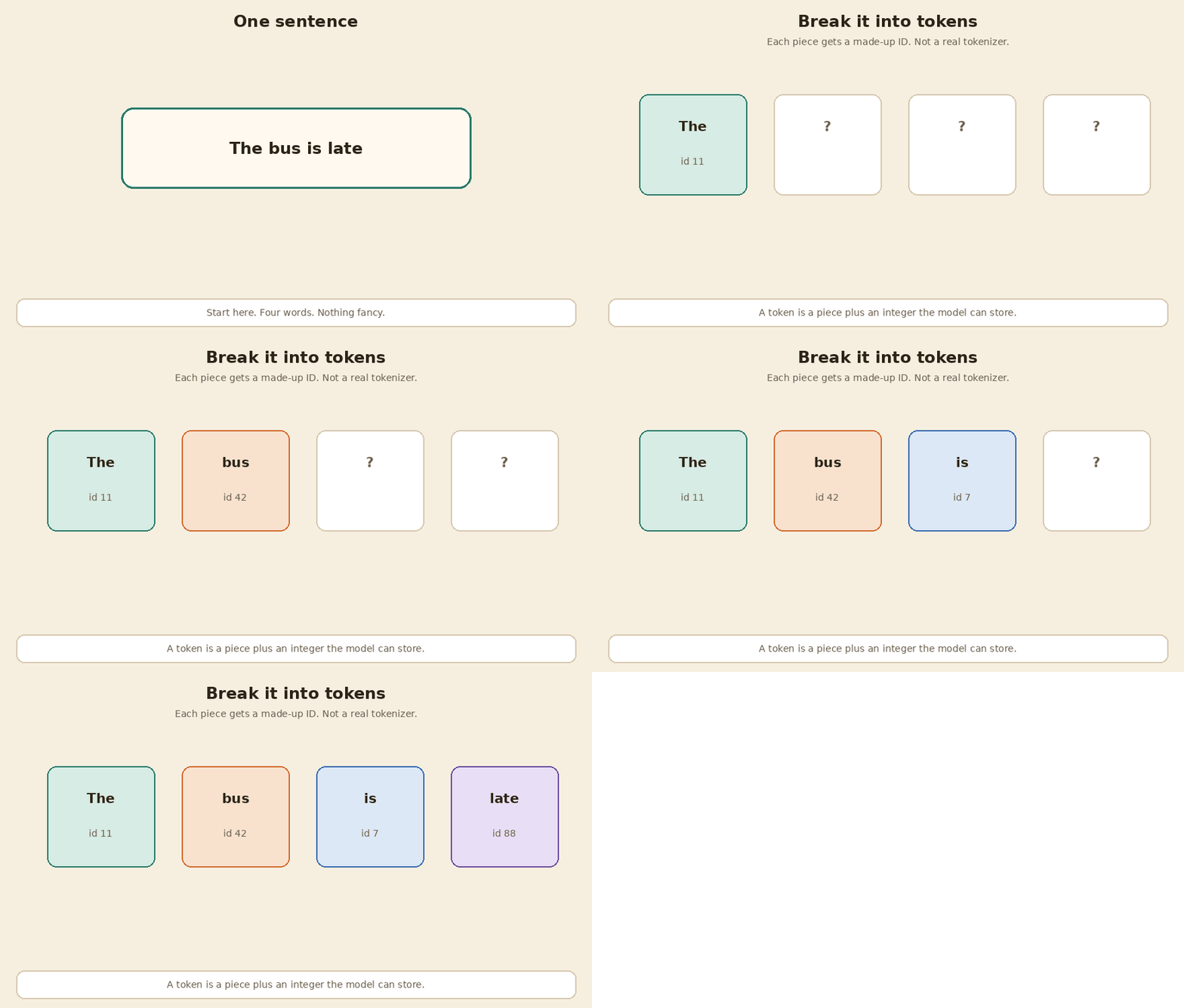
A model does not read English. It reads integers.
A tokenizer cuts text into pieces and maps each piece to an ID. Real systems use tens of thousands of IDs. Here I pick four fake ones so the table stays on one screen.
\[\text{The bus is late} \;\rightarrow\; [(\text{The}, 11),\;(\text{bus}, 42),\;(\text{is}, 7),\;(\text{late}, 88)]\]print("sentence:", SENTENCE)
print("tokens: ", TOKENS)
print("toy ids: ", IDS)
sentence: The bus is late
tokens:   ['The', 'bus', 'is', 'late']
toy ids:  [11 42  7 88]
Those four IDs are invented. Do not look them up in a real vocab.
2. Turn each token into a list of numbers
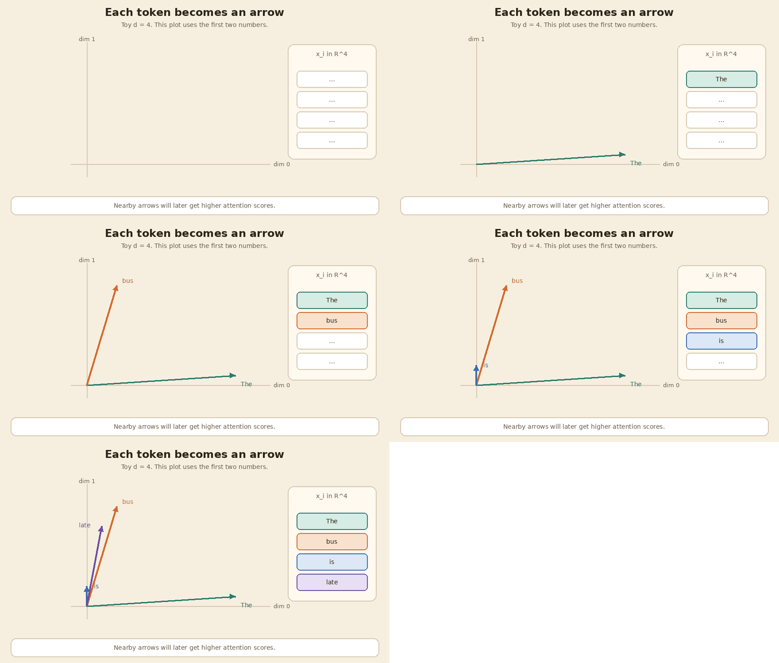
An embedding is a short list of numbers that stands in for a token. Similar tokens sit near each other in that space.
In a real model this list is hundreds of numbers long. Here each token gets 4 numbers. I wrote the table by hand so later dots stay small.
\[x_i \in \mathbb{R}^{4}\]X = np.array(
[
[1.0, 0.1, 0.0, 0.2], # The
[0.2, 1.0, 0.1, 0.3], # bus
[0.0, 0.2, 1.0, 0.1], # is
[0.1, 0.8, 0.0, 1.0], # late
]
)
print(X)
print("shape", X.shape)
[[1.  0.1 0.  0.2]
 [0.2 1.  0.1 0.3]
 [0.  0.2 1.  0.1]
 [0.1 0.8 0.  1. ]]
shape (4, 4)
Four tokens. Four numbers each. Shape (4, 4).
The picture below plots only the first two numbers, so you can see the arrows. bus and late point a similar way. That will matter in a few steps.
3. Let every token ask a question
The query is “what am I looking for, right now?”
You do not invent that question by hand. You multiply the embedding by a learned matrix $W_Q$. Same matrix for every token.
In NumPy the tokens are rows, so the line is Q = X @ W_Q. Same multiply, just a row layout.
W_Q = np.array(
    [
        [0.9, 0.1, 0.0, 0.0],
        [0.0, 0.9, 0.1, 0.0],
        [0.0, 0.0, 0.9, 0.1],
        [0.1, 0.0, 0.0, 0.9],
    ]
)
Q = X @ W_Q
print(Q)
[[0.92 0.19 0.01 0.18]
 [0.21 0.92 0.19 0.28]
 [0.01 0.18 0.92 0.19]
 [0.19 0.73 0.08 0.9 ]]
Row 3 is the query for late: [0.19 0.73 0.08 0.90]. We will use that row next.
4. Give every token a way to answer
The key is the label on the token. The value is the payload you actually mix in if that token gets picked.
Two more matrices. Same idea as the query.
\[k = W_K x,\qquad v = W_V x\]W_K = np.array(
[
[0.8, 0.0, 0.1, 0.1],
[0.1, 0.8, 0.0, 0.1],
[0.0, 0.1, 0.8, 0.1],
[0.1, 0.0, 0.1, 0.8],
]
)
W_V = np.diag([0.6, 0.6, 0.6, 0.6])
K = X @ W_K
V = X @ W_V
print("K")
print(K)
print("V")
print(V)
K
[[0.83 0.08 0.12 0.27]
 [0.29 0.81 0.13 0.37]
 [0.03 0.26 0.81 0.2 ]
 [0.26 0.64 0.11 0.89]]
V
[[0.6  0.06 0.   0.12]
 [0.12 0.6  0.06 0.18]
 [0.   0.12 0.6  0.06]
 [0.06 0.48 0.   0.6 ]]
Three jobs, three lists: $q$, $k$, $v$. Still shape (4, 4).
5. Compare one token’s query with every key
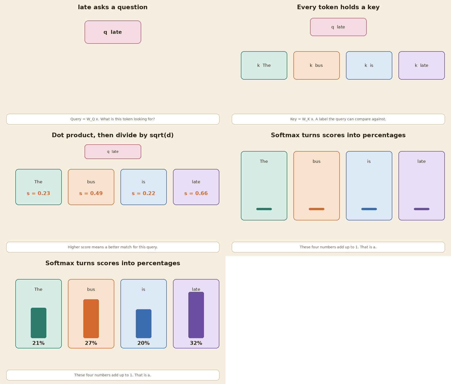
Take the query for late. Dot it with each key. Divide by $\sqrt{d}$ so the numbers do not grow with the width of the list.
A bigger score means a better match.
\[s_j = \frac{q \cdot k_j}{\sqrt{d}}\]q_late = Q[3]
scores = q_late @ K.T / SCALE
print("q_late:", q_late)
print("scores:", scores)
q_late: [0.19 0.73 0.08 0.9 ]
scores: [0.23 0.49 0.22 0.66]
late matches itself most (0.66), then bus (0.49). That fits the embeddings: those two arrows already pointed a similar way.
6. Turn scores into percentages
Softmax makes the four scores positive and forces them to add up to 1.
You can read each weight as “how much of my mix should come from this token?”
\[a_j = \frac{e^{s_j}}{\sum_m e^{s_m}}\]weights = softmax(scores)
print("a = softmax(s):", weights)
print("sum:", weights.sum())
a = softmax(s): [0.21 0.27 0.2  0.32]
sum: 1.0
So late takes 32% from itself, 27% from bus, 21% from The, 20% from is.
7. Mix the values using those weights
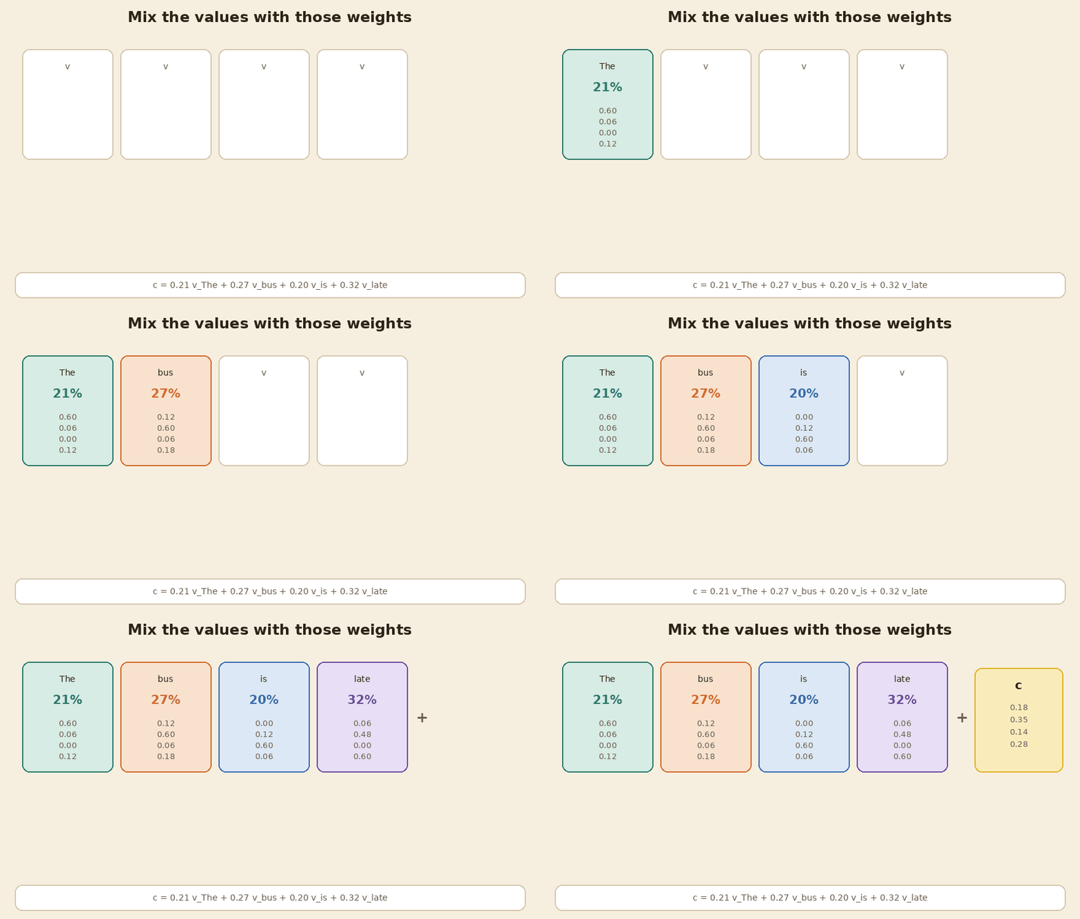
The scores only decide who matters. The values are what you actually add in.
One weighted sum. One new list of four numbers for late.
c = weights @ V
print("c = sum a_j v_j:", c)
c = sum a_j v_j: [0.18 0.35 0.14 0.28]
That is the view late now has of the whole sentence.
8. Do it for every token at once
The last three steps were for one query. The model does the same for every token, in one matrix multiply.
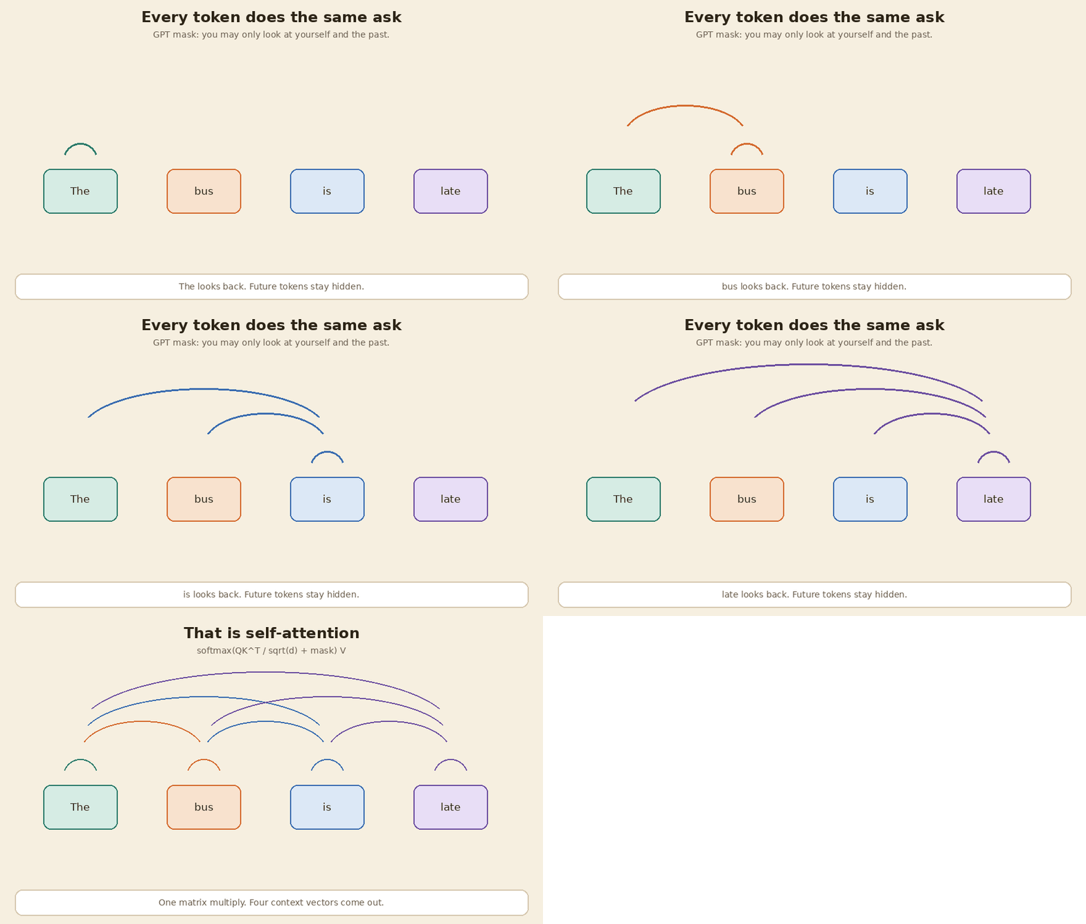
GPT also puts a causal mask on the scores. A token may look at itself and the past. It may not look at a word that has not been written yet. That is how next-word training stays honest.
\[\mathrm{Attention}(Q,K,V) = \mathrm{softmax}\!\left(\frac{QK^{\top}}{\sqrt{d}} + M\right)V\]$M$ is $0$ on and below the diagonal, and $-\infty$ above it. After softmax, the future weights become $0$.
raw = Q @ K.T / SCALE
causal = np.tril(np.ones((4, 4)))
masked = np.where(causal == 1.0, raw, -1e9)
A = softmax(masked, axis=1)
C = A @ V
print("raw scores")
print(raw)
print("causal weights")
print(A)
print("context matrix")
print(C)
raw scores
[[0.41 0.24 0.06 0.26]
 [0.17 0.47 0.23 0.46]
 [0.09 0.17 0.42 0.19]
 [0.23 0.49 0.22 0.66]]
causal weights
[[1.   0.   0.   0.  ]
 [0.43 0.57 0.   0.  ]
 [0.29 0.31 0.4  0.  ]
 [0.21 0.27 0.2  0.32]]
context matrix
[[0.6  0.06 0.   0.12]
 [0.32 0.37 0.03 0.15]
 [0.21 0.25 0.26 0.11]
 [0.18 0.35 0.14 0.28]]
Row 0 is The. It can only see itself, so its weights are [1, 0, 0, 0]. Row 3 is late. It can see everyone. That last row is the same mix we built by hand.
9. Add a small neural network and residual connections
Attention is the talk step. Each token still needs a private think step. That is a tiny MLP, applied at every position with the same weights.
A residual connection adds the input back: $x + \text{layer}(x)$. The original signal still has a path through the stack. Layer norm rescales each token’s numbers so they do not blow up as you go deeper.
\[h = x + \mathrm{Attn}(x),\qquad y = h + \mathrm{MLP}(h)\]H = X + C
W1 = np.array(
[
[0.4, 0.1, 0.0, 0.0],
[0.0, 0.4, 0.1, 0.0],
[0.0, 0.0, 0.4, 0.1],
[0.1, 0.0, 0.0, 0.4],
]
)
W2 = np.array(
[
[0.3, 0.0, 0.1, 0.0],
[0.0, 0.3, 0.0, 0.1],
[0.1, 0.0, 0.3, 0.0],
[0.0, 0.1, 0.0, 0.3],
]
)
mlp = np.maximum(H @ W1, 0.0) @ W2
Y = H + mlp
print("h = X + C")
print(H)
print("y = h + MLP(h)")
print(Y)
h = X + C
[[1.6  0.16 0.   0.32]
 [0.52 1.37 0.13 0.45]
 [0.21 0.45 1.26 0.21]
 [0.28 1.15 0.14 1.28]]
y = h + MLP(h)
[[1.8  0.24 0.07 0.38]
 [0.62 1.57 0.22 0.57]
 [0.3  0.53 1.43 0.3 ]
 [0.36 1.35 0.21 1.48]]
Still shape (4, 4). Same four tokens, richer lists.
10. Stack the blocks
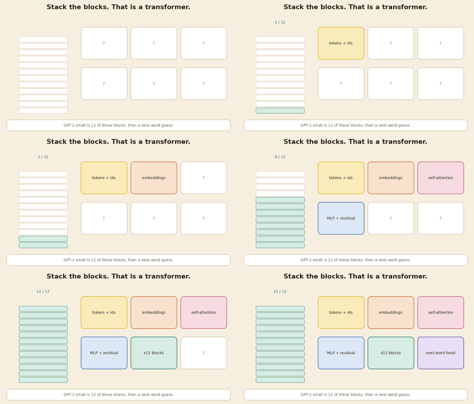
One block is one talk-then-think cycle. A transformer is that cycle repeated.
GPT-2 small does this 12 times. Each block has its own weights. The data shape stays the same as it goes up the stack. In this toy that shape is still (4, 4).
print("GPT-2 small repeats this block 12 times.")
print("toy stack depth: 12")
GPT-2 small repeats this block 12 times.
toy stack depth: 12
We do not run 12 toy blocks here. The idea is the repeat, not a new formula.
11. Train it to predict the next word
After the last block, a linear head turns the last token’s vector into a score per word. Softmax turns those scores into a probability bar.
Three training stages, in plain words:
- Pretraining. Read a huge pile of text. Guess the next token. That is the transformer learning language.
- SFT (supervised fine-tune). Show instruction and answer pairs. Same next-token loss, but now the text looks like a helpful reply.
- RLHF / preference tuning. People pick the better of two answers. The model moves toward the preferred one.
We skip the training loop. We only do the last multiply, with a four-word toy vocab.
\[p(\text{next}) = \mathrm{softmax}(y_{\text{late}}\, W_{\text{head}})\]vocab = ["early", "again", "today", "."]
W_head = np.array(
[
[0.2, 0.1, 0.4, 0.8],
[-0.3, 0.2, 0.6, 0.1],
[0.1, 0.4, 0.2, 0.3],
[0.8, 0.1, 1.2, 0.4],
]
)
logits = Y[3] @ W_head
probs = softmax(logits)
print("logits:", logits)
for word, p in zip(vocab, probs):
bar = "#" * int(round(float(p) * 20))
print(f" {word:6s} {p:4.2f} {bar}")
logits: [0.88 0.54 2.78 1.08]
  early   0.10  ##
  again   0.07  #
  today   0.69  ##############
  .       0.13  ###
| Next word | Probability |
|---|---|
| early | 10% |
| again | 7% |
| today | 69% |
| . | 13% |
On this toy head, the next word after The bus is late is most likely today. Sample from that bar, append the word, run the ladder again. That is how a chat reply gets written: one token at a time.
These percentages are from the tiny matrices above. They are not a real ChatGPT sample.
12. Rewind everything
Take the stack off. Take the block off. Take attention off. You are left with four IDs, then four words.
print("back to the sentence:", SENTENCE)
back to the sentence: The bus is late
That is the whole machine, seen from one short line of English.
Checkpoint recap
| Step | You get | Shape of the data |
|---|---|---|
| 1. Tokens | pieces + toy IDs | 4 ids |
| 2. Embeddings | $x_i \in \mathbb{R}^{4}$ | (4, 4) |
| 3. Query | $q = W_Q x$ | (4, 4) |
| 4. Key and value | $k = W_K x$, $v = W_V x$ | (4, 4) each |
| 5. Scores | $s_j = q \cdot k_j / \sqrt{d}$ | (4,) for one query |
| 6. Weights | softmax of the scores | (4,), sums to 1 |
| 7. Context | $c = \sum a_j v_j$ | (4,) |
| 8. Self-attention | $\mathrm{softmax}(QK^{\top}/\sqrt{d}+M)V$ | (4, 4) |
| 9. Transformer block | $h = x + \mathrm{Attn}(x)$, $y = h + \mathrm{MLP}(h)$ | (4, 4) |
| 10. Transformer | 12 stacked blocks (GPT-2 small) | still (4, 4) in this toy |
| 11. Chat assistant | next-word bar, then SFT + preference | (4,) over the toy vocab |
| 12. Rewind | the original sentence | text |
In short
The bus is late becomes four toy IDs, then four short lists of numbers. Those lists ask questions (query), wear labels (key), and carry a payload (value). One token’s query is scored against every key, squashed into percentages, and used to mix the values. Do that for every token, hide the future with a causal mask, and you have self-attention. Add a small MLP and residual links and you have one transformer block. Stack twelve of those and you have a GPT-shaped model. Train it to guess the next word, then fine-tune with instructions and human preference, and you have the same idea that sits under ChatGPT. Undo the steps and you are back at the sentence.
If this helped:

Discussion
Reactions and replies via GitHub Discussions. Sign in with GitHub to comment.